Partitioning a Pipeline

Here’s a simple use case for applying connectivity constraints in Hierarchical Clustering. Our goal is to partition a raster image of the Canadian pipeline such that all pixels in a cluster will be connected through a sequence of adjacent members.

See here for the data source: https://ssc.ca/en/case-study/what-geographical-factors-are-associated-pipeline-incidents-involve-spills

import numpy as np
import pandas as pd
import matplotlib.pyplot as plt 

from collections import deque
from scipy.spatial.distance import cdist
from sklearn.cluster import AgglomerativeClustering

img = plt.imread('gdm-Pipelines_EN.png')
fig, ax = plt.subplots(figsize=(10,10))
plt.imshow(img);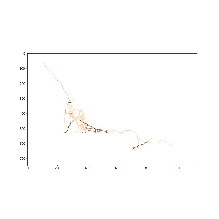

Let’s ignore any information colour is providing here and convert to a binary image. We’ll also crop out any unnecessary whitespace.

# convert to binary image
pixels = img[:,:,3] > 0

# crop out whitespace
bot_crop = np.argmax(pixels.max(axis=1))
top_crop = pixels.shape[0] - np.argmax(pixels.max(axis=1)[::-1])
left_crop = np.argmax(pixels.max(axis=0))
right_crop = pixels.shape[1] - np.argmax(pixels.max(axis=0)[::-1])
pixels = pixels[bot_crop:top_crop,left_crop:right_crop]

plt.imshow(pixels,cmap='binary');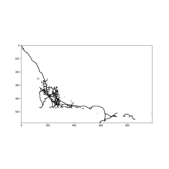

Now let’s convert the raster to a graph where each node represents a coloured cell and each edge indicates two cells that are adjacent by a queen’s move one cell away.

Scikit-learn’s AgglomerativeClustering requires a connected graph so we’ll need to determine all the disconnected components using breadth-first search. Then we’ll use Kruskal’s algorithm to find the minimum spanning tree that connects all components and add those edges to the adjacency matrix.

# convert nonempty cells to nodes
nodes = np.array(np.where(pixels == 1)).T
n_nodes = len(nodes)

# create adjacency matrix by assigning edges to adjacent pixels
dist_matrix = cdist(nodes,nodes)
adj_matrix = 1*(dist_matrix<2)

# find all disconnected components
component_labels = np.zeros(n_nodes) - 1
componentId = 0
Q = deque()
for i in range(len(nodes)):
    if component_labels[i] == -1:
        component_labels[i] = componentId
        Q.append(i)
        while len(Q) > 0:       
            for j in np.where(adj_matrix[Q[0]] == 1)[0]:
                if component_labels[j] == -1:
                    component_labels[j] = componentId
                    Q.append(j)
            Q.popleft()
        componentId += 1

# for each pair of disconnected components find the edge w/ min distance to connect 
comp_edges = []
for i in range(componentId-1):
    for j in range(i+1,componentId):
        i_nodes = np.where(component_labels == i)[0]
        j_nodes = np.where(component_labels == j)[0]
        btwn_comps_matrix = dist_matrix[np.ix_(i_nodes, j_nodes)]
        min_dist_matrix_coords = np.unravel_index(btwn_comps_matrix.argmin(),btwn_comps_matrix.shape)
        comp_edges.append(
            [
                [i,j], # edge: component ids
                btwn_comps_matrix[min_dist_matrix_coords], # distance
                [i_nodes[min_dist_matrix_coords[0]],j_nodes[min_dist_matrix_coords[1]]], # edge: node ids
            ]
        )
comp_edges = sorted(comp_edges, key=lambda i: i[1])

# Kruskal's Algorithm - Find Min Spanning Tree to reconnect entire graph
comp_connectors = []
joined_comp_labels = np.arange(componentId)
for edge in comp_edges:
    if joined_comp_labels[edge[0][0]] != joined_comp_labels[edge[0][1]]:
        joined_comp_labels[np.where(joined_comp_labels==joined_comp_labels[edge[0][1]])] = joined_comp_labels[edge[0][0]]
        comp_connectors.append(edge[-1])

# connect adjacency matrix
connected_adj_matrix = adj_matrix.copy()
for edge in comp_connectors:
    connected_adj_matrix[edge[0], edge[1]] = 1
    connected_adj_matrix[edge[1], edge[0]] = 1

fig, ax = plt.subplots(figsize=(20,20))
plt.imshow(pixels,cmap='binary',alpha=.1)
for i in range(len(comp_connectors)):
    pixel_coords = nodes[comp_connectors[i]]
    plt.plot(pixel_coords[:,1],pixel_coords[:,0],linewidth=5);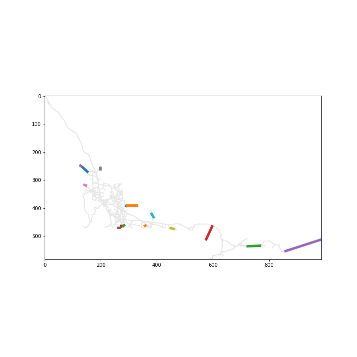

It’s time to partition the pipeline.

n_clusters = 74  # number of regions
ward = AgglomerativeClustering(
   n_clusters=74, linkage="ward", connectivity=connected_adj_matrix
)
model = ward.fit(nodes)

Let’s create a network from the partitioned regions. We’ll need to find which clusters are adjacent.

# create centroids for each cluster
centers = []
for i in range(n_clusters):
    centers.append(nodes[np.where(ward.labels_ == i)].mean(axis=0))
centers = np.array(centers)

# find adjacent clusters
dist_btwn_clusters = np.zeros((n_clusters,n_clusters))
for i in range(n_clusters-1):
    for j in range(i+1,n_clusters):
        i_nodes = np.where(ward.labels_ == i)[0]
        j_nodes = np.where(ward.labels_ == j)[0]
        dist_btwn_clusters[i,j] = dist_matrix[np.ix_(i_nodes, j_nodes)].min()
        dist_btwn_clusters[j, i] = dist_btwn_clusters[i, j]

clusters_adj_matrix = (dist_btwn_clusters < 2)
np.fill_diagonal(clusters_adj_matrix, False)

plt.figure(figsize=(18,16))
plt.imshow(pixels,cmap='binary',alpha=0)
plt.scatter(nodes[:,1], nodes[:,0], c=ward.labels_, s=0.5, cmap='jet',alpha=0.2)
plt.scatter(centers[:,1], centers[:,0], c='k', s=30);

edges = np.where(clusters_adj_matrix)
for i in range(len(edges[0])):
    plt.plot(
        [centers[edges[0][i],1],centers[edges[1][i],1]],
        [centers[edges[0][i],0],centers[edges[1][i],0]],
        c='k'
    )

And that’s it! As a bonus the source provided some oilspill data. Let’s check where they occur. Oilspill coordinates are in latitude and longitude so we’ll have to convert it to our image’s coordinates using a mercator projection. The function below is derived from https://en.wikipedia.org/wiki/Mercator_projection#Mathematics

def convertGeoCordsToPixel(
        coordinates,
        pixelWidth, 
        pixelHeight, 
        longLeftmostPixel, 
        longRightmostPixel, 
        latSouthmostPixel):
    latitudes = coordinates[:,0]
    longitudes = coordinates[:,1]

    pixelperLongDegree = (pixelWidth / (longRightmostPixel - longLeftmostPixel))
    entireWorldWidth = pixelperLongDegree * 360
    globeRadius =  entireWorldWidth / (2 * np.pi)

    x = globeRadius * np.pi / 180 * (longitudes - longLeftmostPixel)

    latitudes_Rad = latitudes * np.pi / 180 
    latSouthmostPixel_Rad = latSouthmostPixel * np.pi / 180 
    yOffset = globeRadius / 2 * np.log((1 + np.sin(latSouthmostPixel_Rad)) / (1 - np.sin(latSouthmostPixel_Rad)))
    y = (yOffset + pixelHeight) - globeRadius / 2 * np.log((1 + np.sin(latitudes_Rad)) / (1 - np.sin(latitudes_Rad))) 
    
    return np.array([y, x]).T

oilspills = pd.read_csv('oilspills.csv')
spill_latlong = oilspills[['Latitude','Longitude']].values

spill_coords = convertGeoCordsToPixel(
    spill_latlong,
    pixels.shape[1],
    pixels.shape[0], 
    -134.9, 
    -48.5, 
    42
) 

plt.figure(figsize=(10,10))
plt.imshow(pixels, cmap='binary', alpha=.2)
plt.scatter(spill_coords[:,1], spill_coords[:,0], ec='k', alpha=.5);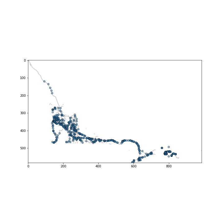

Looks close enough. Finally, let’s assign each spill to the closest cluster.

oilspills['cluster'] = ward.labels_[cdist(spill_coords, nodes).argmin(axis=1)]
spill_labels = oilspills['cluster'].values.tolist()
spills_counts = [spill_labels.count(i) for i in range(n_clusters)]

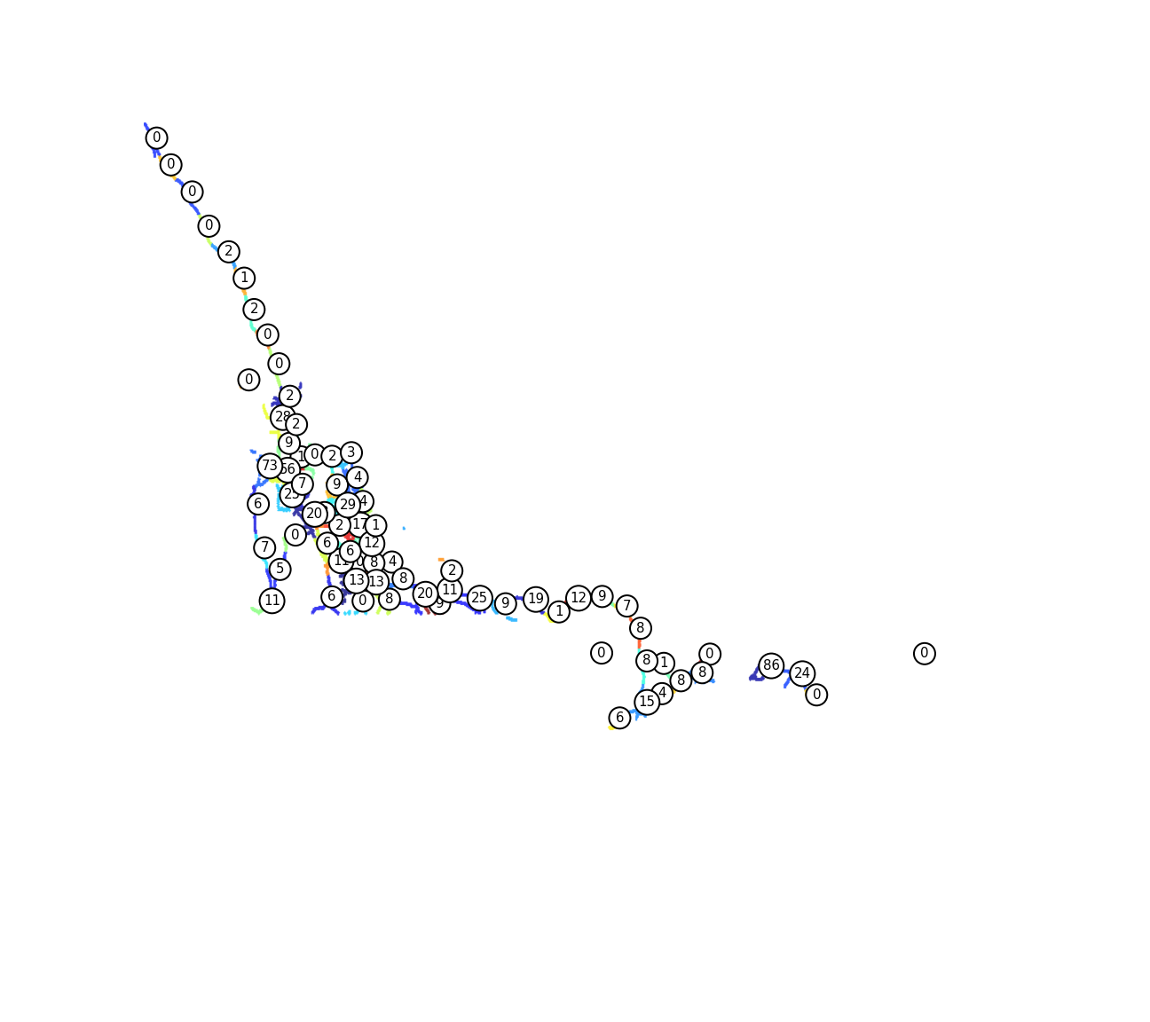
plt.figure(figsize=(18,16))
plt.xlim(0,img.shape[1])
plt.ylim(-img.shape[0],0)
plt.scatter(nodes[:,1], -nodes[:,0],c=ward.labels_, s=0.5, cmap='jet',alpha=0.5,zorder=-100000000)
plt.scatter(centers[:,1], -centers[:,0],c='k', s=25,zorder=-10000000);
for i in range(len(centers)):
    plt.annotate(spills_counts[i],(centers[i,1],-centers[i,0]),size=15,bbox=dict(boxstyle="circle,pad=0.3", fc='w', ec="k", lw=2),zorder=-i)
plt.axis('off');